Estimation and Prediction of the Wet Season Calendar (WSC) Using a Daily Soil Water Balance Model for Agricultural Applications Using ``AquaBEHER``

1. Introduction

Welcome to the tutorial for AquaBEHER, an R package designed to estimate and predict the wet season calendar and soil water balance for agricultural applications. This vignette provides a practical guide to using AquaBEHER. The package integrates daily potential evapotranspiration (PET) and soil water balance parameters to compute the wet season calendar (WSC) for crop and soil water management. Using these parameters, AquaBEHER can estimate and predict the onset, cessation, and duration of the wet season based on an agroclimatic approach.

In this tutorial, you will learn how to:

Install and set up AquaBEHER.
Estimate potential evapotranspiration (PET) using different methods.
Calculate daily soil water balance.
Estimate the wet season calendar using an agroclimatic approach.

2. Installation and Loading

To install the latest development version of AquaBEHER, use devtools. Ensure that Rtools is installed on Windows for full functionality.

## Install required packages:
# if (!require("pacman")) install.packages("pacman")
# pacman::p_load(knitr, rmarkdown, prettydoc, dplyr, ggplot2, lubridate,
# terra, devtools, ggrepel, zoo)

## Install AquaBEHER from CRAN:
# install.packages("AquaBEHER")

## Install AquaBEHER from GitHub:
# devtools::install_github("RobelTakele/AquaBEHER")

library(AquaBEHER)
library(ggplot2)
library(ggrepel)
library(dplyr)

3. Required Climate Data

For evapotranspiration calculations, various meteorological and geographical parameters are needed, as shown below:

Meteorological Data:

Maximum and minimum temperature
Solar radiation
Dew point temperature
Wind speed
Rainfall

Geographical Data:

Latitude
Longitude
Elevation

data(AgroClimateData)
str(AgroClimateData)
#> 'data.frame':    14975 obs. of  14 variables:
#>  $ GridID: chr  "MOZ0007149" "MOZ0007149" "MOZ0007149" "MOZ0007149" ...
#>  $ Lat   : num  -15.1 -15.1 -15.1 -15.1 -15.1 ...
#>  $ Lon   : num  39.3 39.3 39.3 39.3 39.3 ...
#>  $ Elev  : num  392 392 392 392 392 ...
#>  $ WHC   : num  97.8 97.8 97.8 97.8 97.8 ...
#>  $ Year  : num  1982 1982 1982 1982 1982 ...
#>  $ Month : num  1 1 1 1 1 1 1 1 1 1 ...
#>  $ Day   : num  1 2 3 4 5 6 7 8 9 10 ...
#>  $ Rain  : num  0 0 0 1.91 0 ...
#>  $ Tmax  : num  32.2 33.1 33.5 32.8 32.7 ...
#>  $ Tmin  : num  23.1 23.1 23.1 23.6 22.8 ...
#>  $ Rs    : num  23.9 26.4 25 24.2 23.4 ...
#>  $ Tdew  : num  20.2 20.5 20.5 20.8 21.4 ...
#>  $ Uz    : num  4.72 4.28 3.62 2.54 1.48 ...
head(AgroClimateData)
#>       GridID       Lat     Lon     Elev      WHC Year Month Day     Rain
#> 1 MOZ0007149 -15.09238 39.2519 392.1337 97.84914 1982     1   1 0.000000
#> 2 MOZ0007149 -15.09238 39.2519 392.1337 97.84914 1982     1   2 0.000000
#> 3 MOZ0007149 -15.09238 39.2519 392.1337 97.84914 1982     1   3 0.000000
#> 4 MOZ0007149 -15.09238 39.2519 392.1337 97.84914 1982     1   4 1.907393
#> 5 MOZ0007149 -15.09238 39.2519 392.1337 97.84914 1982     1   5 0.000000
#> 6 MOZ0007149 -15.09238 39.2519 392.1337 97.84914 1982     1   6 0.000000
#>       Tmax     Tmin       Rs     Tdew       Uz
#> 1 32.24396 23.11500 23.86698 20.21160 4.723783
#> 2 33.07202 23.12585 26.38375 20.48284 4.279407
#> 3 33.49679 23.12602 25.00704 20.45689 3.622179
#> 4 32.76818 23.60351 24.16475 20.83896 2.535047
#> 5 32.65872 22.79294 23.44483 21.36882 1.477617
#> 6 31.80630 22.43975 21.99277 21.29297 1.953415

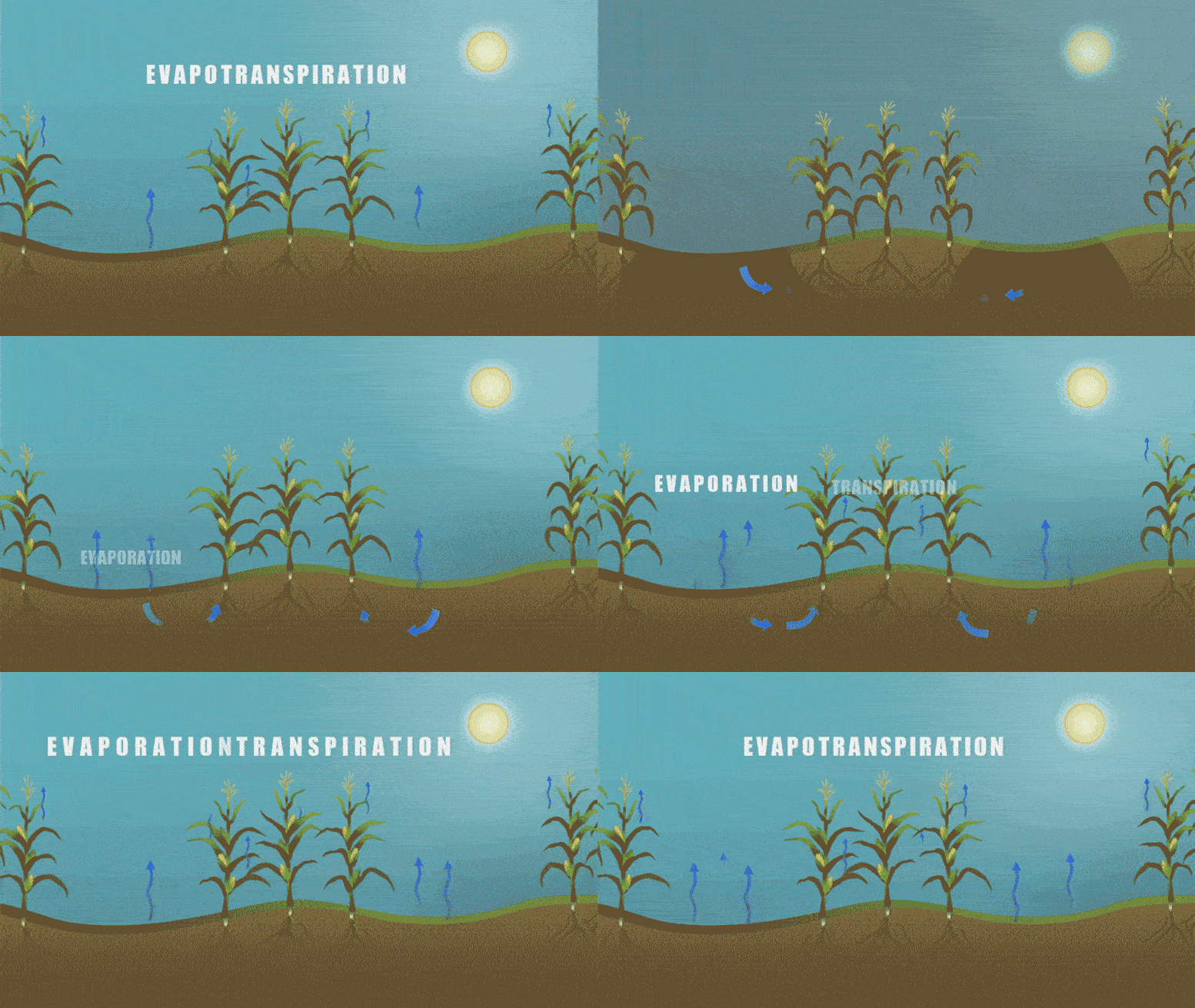
4. Potential Evapotranspiration

Potential evapotranspiration (PET) is vital for agricultural water management. AquaBEHER offers multiple methods to estimate PET, including the FAO Penman-Monteith, Priestley-Taylor, and Hargreaves-Samani formulations.

Evapotranspiration cycle

Usage:

PET <- calcEto(AgroClimateData, method = “PM”, crop = “short”)
str(PET)

The function return a list of
- daily estimations of PET in (mm/day)
- daily estimations of extraterrestrial radiation (MJ/m2/day)
- daily estimations of slope of vapor pressure curve (kPa/°C)

Example:

The calcEto function computes PET with inputs of a data frame containing daily values of meteorological parameters:

PET <- calcEto(AgroClimateData, method = "PM", crop = "short")

str(PET)
#> List of 7
#>  $ ET.Daily      : num(0) 
#>  $ Ra.Daily      : num [1:14975] 40.9 40.9 40.9 40.9 40.9 ...
#>  $ Slope.Daily   : num [1:14975] 0.217 0.221 0.224 0.222 0.217 ...
#>  $ Ea.Daily      : num [1:14975] 2.37 2.41 2.41 2.46 2.54 ...
#>  $ Es.Daily      : num [1:14975] 3.82 3.94 4 3.94 3.85 ...
#>  $ ET.formulation: chr "Penman-Monteith FAO56"
#>  $ ET.type       : chr "Reference Crop ET"
#>  - attr(*, "class")= chr "PEToutList"

Graphical comparison of the evapotranspiration (mm/day) calculated using the FAO Penman–Monteith formulation and the Hargreaves-Samani formulation:

## Compute PET using Hargreaves-Samani formulation using the sample data f
## rom 'AgroClimateData':
Eto.HS <- calcEto(AgroClimateData, method = "HS")

## Now compute PET using Penman-Monteith formulation:
Eto.PM <- calcEto(AgroClimateData, method = "PM", Zh = 10)

plot(Eto.PM$ET.Daily[1:1000],
  type = "l", xlab = "Days since 1996",
  ylab = "Eto (mm/day)", col = "black", lwd = 1, lty = 2
)
lines(Eto.HS$ET.Daily[1:1000], col = "blue", lwd = 2, lty = 1)

legend("bottom", c("Eto: Penman–Monteith", "Eto: Hargreaves-Samani"),
  horiz = TRUE, bty = "n", cex = 1, lty = c(2, 1),
  lwd = c(2, 2), inset = c(1, 1),
  xpd = TRUE, col = c("black", "blue")
)

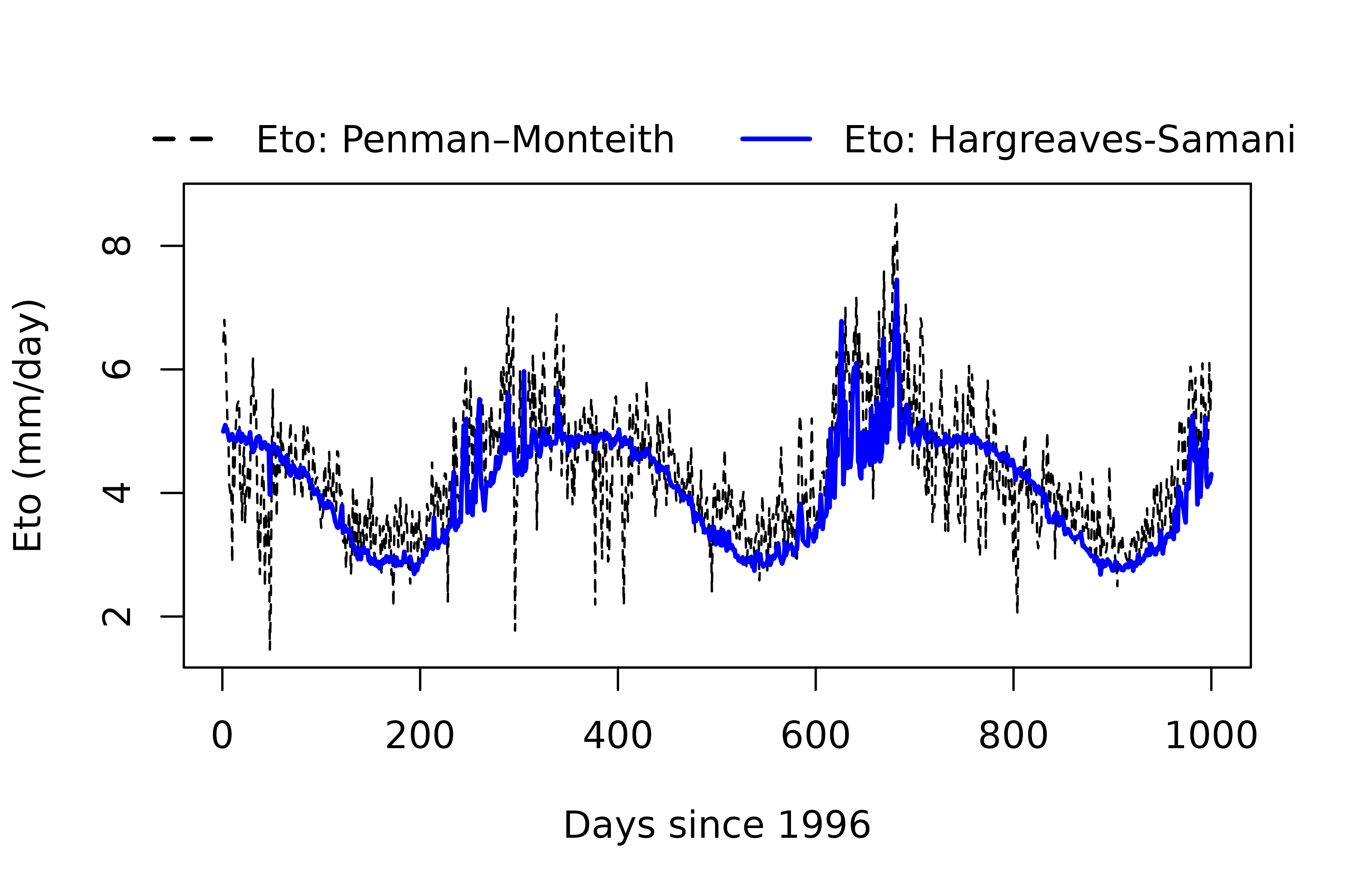
Key Insight: The FAO Penman–Monteith formulation presents enhanced day-to-day variations of evapotranspiration compared to the Hargreaves-Samani formulation.

5. Soil Water Balance

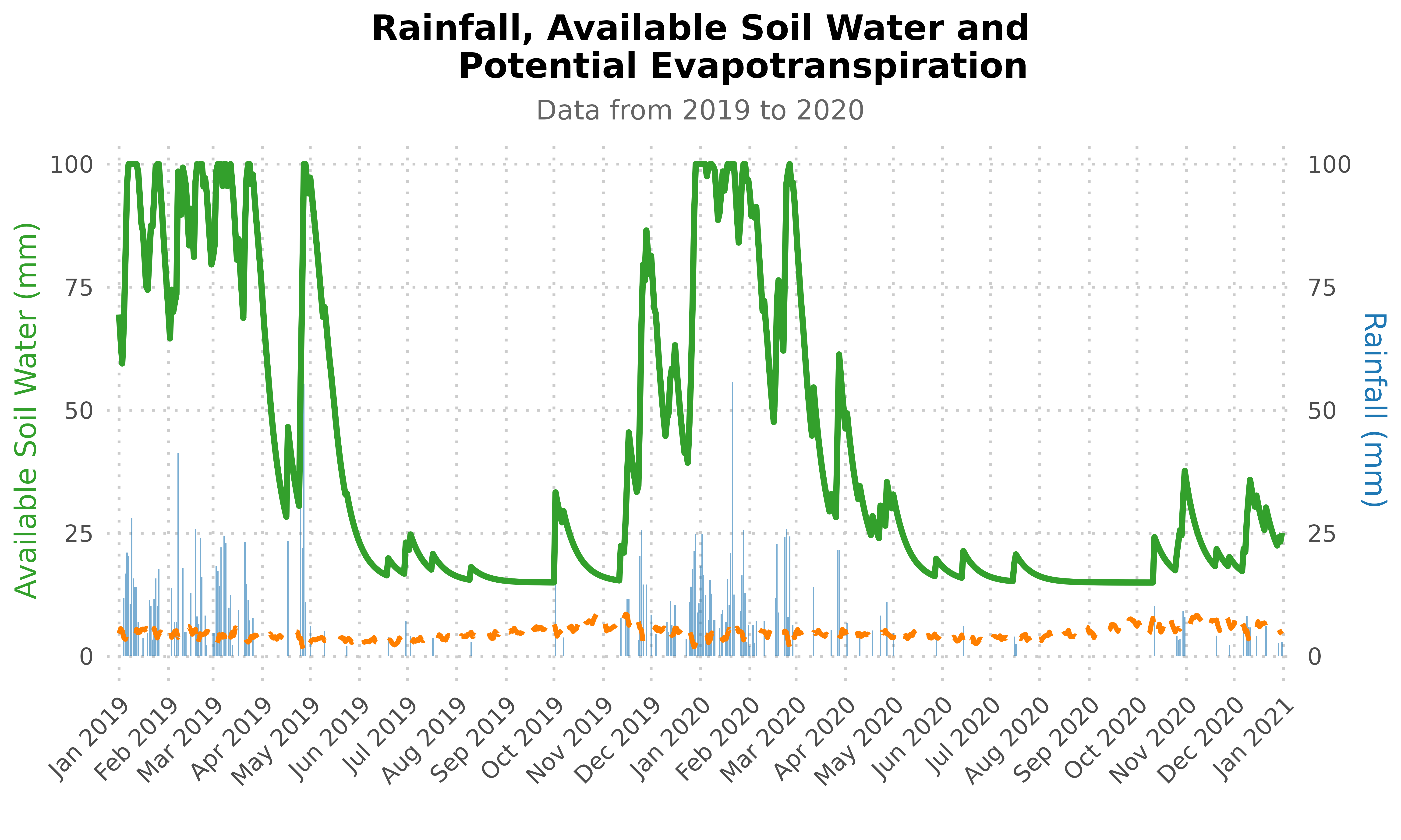
This function performs daily computations of soil water balance parameters for the root zone. Soil water changes daily in response to rainfall, evapotranspiration, runoff and deep drainage.

Assumptions

Atmospheric conditions affect the rate at which crops use water.
The soil has uniform cross-section of homogeneous volume with a measured depth and a unit area.
A well-established, dense grass crop is growing, which completely covers the soil surface.

Usage:

calcWatBal(data, soilWHC)

Example:

The calcWatBal compute with inputs of data frame containing daily values of Rain, Eto and soil water holding capacity.

PET <- calcEto(AgroClimateData, method = "PM", Zh = 10)

## Add the estimated PET 'ET.Daily' to a new column in AgroClimateData:
AgroClimateData$Eto <- PET$ET.Daily

## Estimate daily water balance for the soil having 100mm of soilWHC:
soilWHC <- 100

watBal.list <- calcWatBal(data = AgroClimateData, soilWHC)
watBal <- watBal.list$data

str(watBal)
#> 'data.frame':    14975 obs. of  20 variables:
#>  $ GridID: chr  "MOZ0007149" "MOZ0007149" "MOZ0007149" "MOZ0007149" ...
#>  $ Lat   : num  -15.1 -15.1 -15.1 -15.1 -15.1 ...
#>  $ Lon   : num  39.3 39.3 39.3 39.3 39.3 ...
#>  $ Elev  : num  392 392 392 392 392 ...
#>  $ WHC   : num  97.8 97.8 97.8 97.8 97.8 ...
#>  $ Year  : num  1982 1982 1982 1982 1982 ...
#>  $ Month : num  1 1 1 1 1 1 1 1 1 1 ...
#>  $ Day   : num  1 2 3 4 5 6 7 8 9 10 ...
#>  $ Rain  : num  0 0 0 0 0 ...
#>  $ Tmax  : num  32.2 33.1 33.5 32.8 32.7 ...
#>  $ Tmin  : num  23.1 23.1 23.1 23.6 22.8 ...
#>  $ Rs    : num  23.9 26.4 25 24.2 23.4 ...
#>  $ Tdew  : num  20.2 20.5 20.5 20.8 21.4 ...
#>  $ Uz    : num  4.72 4.28 3.62 2.54 1.48 ...
#>  $ Eto   : num  6.45 6.8 6.49 5.84 5.23 ...
#>  $ R     : num  0 0 0 0 0 0 0 0 0.656 1 ...
#>  $ AVAIL : num  0 0 0 0 0 ...
#>  $ TRAN  : num  0 0 0 0 0 ...
#>  $ DRAIN : num  0 0 0 0 0 0 0 0 0 0 ...
#>  $ RUNOFF: num  0 0 0 0 0 ...

## Filter the data for the years 2019 and 2020:
watBal.19T20 <- watBal[watBal$Year %in% c(2019, 2020), ]

## Create a date vector:
date.vec <- as.Date(paste0(
  watBal.19T20$Year, "-",
  watBal.19T20$Month, "-",
  watBal.19T20$Day
), format = "%Y-%m-%d")

## Add the date vector to the data frame:
watBal.19T20$date <- date.vec

## Plotting the water balance output for the climatological year
## from 2019 to 2020 using ggplot2:

library(ggplot2)
library(scales)

ggplot(data = watBal.19T20, aes(x = date)) +
  geom_bar(aes(y = Rain),
    stat = "identity", fill = "#1f78b4",
    alpha = 0.6, width = 0.8
  ) +
  geom_line(aes(y = AVAIL), color = "#33a02c", size = 1.5) +
  geom_line(aes(y = Eto),
    color = "#ff7f00", size = 1.2,
    linetype = "dashed"
  ) +
  scale_x_date(
    date_labels = "%b %Y", date_breaks = "1 month",
    expand = c(0.01, 0)
  ) +
  scale_y_continuous(
    name = "Available Soil Water (mm)",
    sec.axis = sec_axis(~., name = "Rainfall (mm)")
  ) +
  labs(
    title = "Rainfall, Available Soil Water and
       Potential Evapotranspiration",
    subtitle = "Data from 2019 to 2020",
    x = " ",
    y = " "
  ) +
  theme_minimal(base_size = 15) +
  theme(
    plot.title = element_text(face = "bold", size = 18, hjust = 0.5),
    plot.subtitle = element_text(size = 14, hjust = 0.5, color = "grey40"),
    axis.title.y = element_text(color = "#33a02c"),
    axis.title.y.right = element_text(color = "#1f78b4"),
    axis.text.x = element_text(angle = 45, hjust = 1),
    panel.grid.minor = element_blank(),
    panel.grid.major = element_line(linetype = "dotted", color = "grey80")
  )

6. Rainy Season Calendar

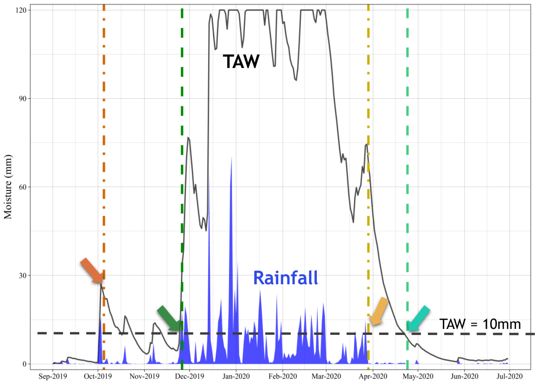
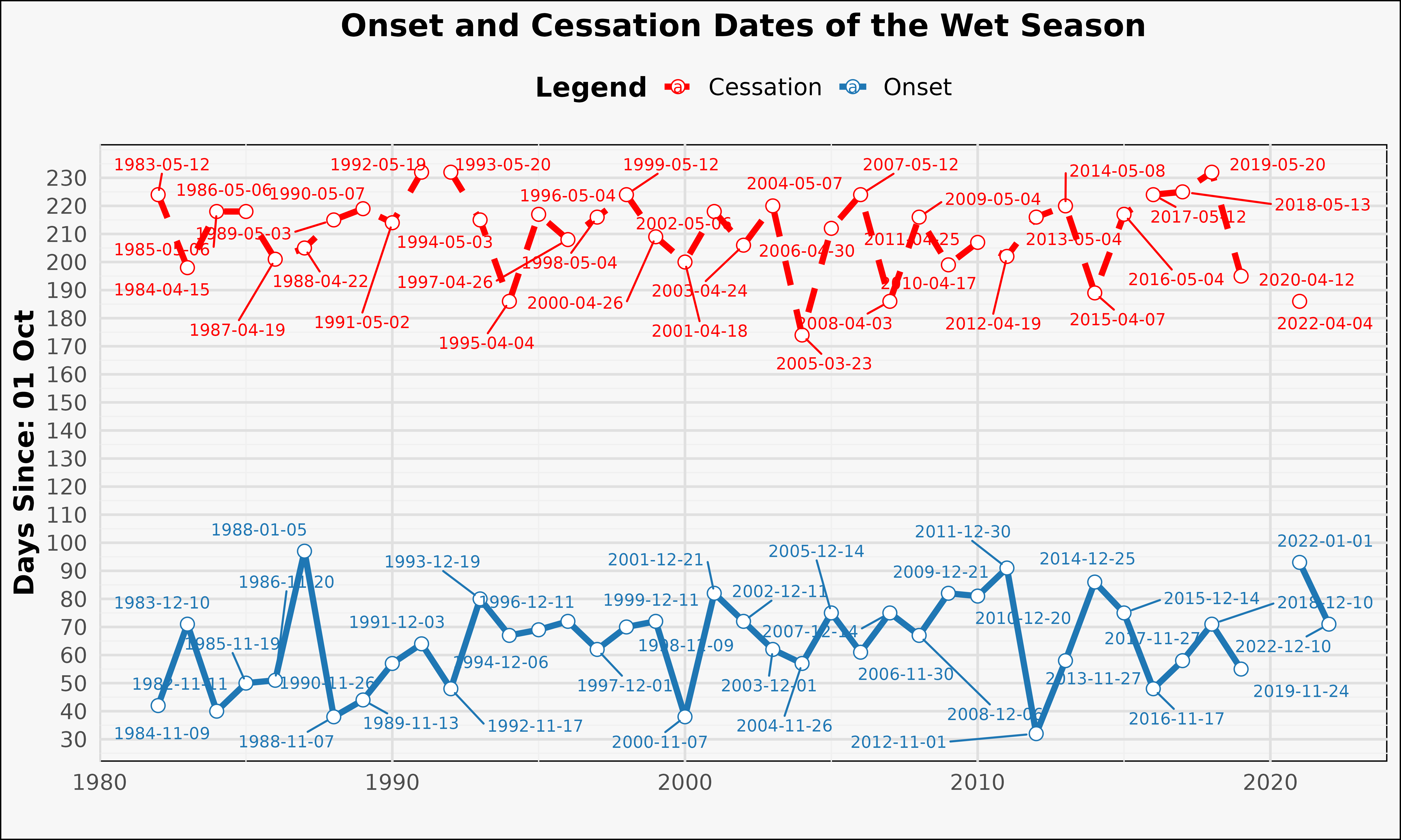
The onset and cessation dates of the wet season were determined for each climatological year Figure 1. The term climatological year represents the period between two driest periods, which is traditionally defined based on a calendar year starting from the driest month and has a fixed length of 12 months.

Figure 1. Example of a climatological yea, the onset and cessation windows

Various methods have been developed to estimate the wet season calendar, i.e. the onset, cessation and duration of the wet season. Common method used for crop production applications is the agroclimatic approach. As per agroclimatic approach, a normal wet season (growing season) is defined as one when there is an excess of precipitation over potential evapotranspiration (PET). Such a period meets the evapotranspiration demands of crops and recharge the moisture of the soil profile (FAO 1977; 1978; 1986). Thus, the wet season calendar defined accordingly:

Onset

The onset of the wet season will start on the first day after onsetWind.start, when the actual-to-potential evapotranspiration ratio is greater than 0.5 for 7 consecutive days, followed by a 20-day period in which plant available water remains above wilting over the root zone of the soil layer.

Cessation

The wet season will end, cessation, on the first day after onsetWind.end, when the actual-to-potential evapotranspiration ratio is less than 0.5 for 7 consecutive days, followed by 12 consecutive non-growing days in which plant available water remains below wilting over the root zone of the soil layer.

Duration

The duration of the wet season is the total number of days from onset to cessation of the season.

Figure 2. Hypothetical example of onset and cessation date determination

Usage:

calcSeasCal(data, onsetWind.start, onsetWind.end, cessaWind.end, soilWHC)

Example:

Using the sample climate data provided by the AquaBEHER package, compute the wet season calendar:

## The wet season calendar is estimated for the onset window ranges from
## 01-September to 31-January having a soil with 80mm of soilWHC:

data(AgroClimateData)

PET <- calcEto(AgroClimateData, method = "HS")
AgroClimateData$Eto <- PET$ET.Daily

soilWHC <- 80

watBal.list <- calcWatBal(data = AgroClimateData, soilWHC)
watBal <- watBal.list$data

onsetWind.start <- "10-01" ## earliest possible start date of the onset window
onsetWind.end <- "01-31" ## the latest possible date for end of the onset window
cessaWind.end <- "06-30" ## the latest possible date for end of the cessation window

seasCal.dF <- calcSeasCal(
  data = watBal, onsetWind.start,
  onsetWind.end, cessaWind.end, soilWHC
)

str(seasCal.dF)
#> 'data.frame':    41 obs. of  8 variables:
#>  $ Year          : num  1982 1983 1984 1985 1986 ...
#>  $ OnsetDate     : Date, format: "1982-11-11" "1983-12-10" ...
#>  $ OnsetDOY      : chr  "315" "344" "314" "323" ...
#>  $ OnsetValue    : int  42 71 40 50 51 97 38 44 57 64 ...
#>  $ CessationDate : Date, format: "1983-05-12" "1984-04-15" ...
#>  $ CessationDOY  : chr  "132" "106" "126" "126" ...
#>  $ CessationValue: int  224 198 218 218 201 205 215 219 214 232 ...
#>  $ Duration      : num  182 127 178 168 150 108 177 175 157 168 ...

seasCal.dF$OnsetDate <- as.Date(seasCal.dF$OnsetDate)
seasCal.dF$CessationDate <- as.Date(seasCal.dF$CessationDate)

max_onset <- max(seasCal.dF$OnsetValue, na.rm = TRUE)
max_cessation <- max(seasCal.dF$CessationValue, na.rm = TRUE)
max_value <- max(max_onset, max_cessation)



ggplot(seasCal.dF, aes(x = Year)) +
  geom_line(aes(y = OnsetValue, color = "Onset"),
    size = 1.5, linetype = "solid"
  ) +
  geom_line(aes(y = CessationValue, color = "Cessation"),
    size = 1.5, linetype = "dashed"
  ) +
  geom_point(aes(y = OnsetValue, color = "Onset"),
    size = 3,
    shape = 21, fill = "white"
  ) +
  geom_point(aes(y = CessationValue, color = "Cessation"),
    size = 3, shape = 21, fill = "white"
  ) +
  geom_text_repel(
    aes(
      y = OnsetValue,
      label = ifelse(!is.na(OnsetDate),
        format(OnsetDate, "%Y-%m-%d"), ""
      ),
      color = "Onset"
    ),
    size = 3,
    box.padding = 0.5, point.padding = 0.5
  ) +
  geom_text_repel(
    aes(
      y = CessationValue,
      label = ifelse(!is.na(CessationDate),
        format(CessationDate, "%Y-%m-%d"), ""
      ),
      color = "Cessation"
    ),
    size = 3,
    box.padding = 0.5, point.padding = 0.5
  ) +
  scale_y_continuous(
    name = paste0(
      "Days Since: ",
      format(
        as.Date(paste0(
          "2023-",
          onsetWind.start
        )),
        "%d %b"
      )
    ),
    breaks = seq(0, max_value, by = 10)
  ) +
  labs(
    title = "Onset and Cessation Dates of the Wet Season",
    x = " ", color = "Legend"
  ) +
  theme_minimal(base_size = 14) +
  theme(
    plot.title = element_text(hjust = 0.5, face = "bold", size = 16),
    legend.position = "top",
    axis.title.x = element_text(face = "bold"),
    axis.title.y = element_text(face = "bold"),
    legend.title = element_text(face = "bold"),
    legend.text = element_text(size = 12),
    panel.grid.major = element_line(color = "#e0e0e0"),
    panel.grid.minor = element_line(color = "#f0f0f0"),
    panel.background = element_rect(fill = "#f7f7f7"),
    plot.background = element_rect(fill = "#f7f7f7")
  ) +
  scale_color_manual(
    name = "Legend",
    values = c(
      "Onset" = "#1f77b4",
      "Cessation" = "red"
    )
  )

7. Seasonal Forecast of WSC

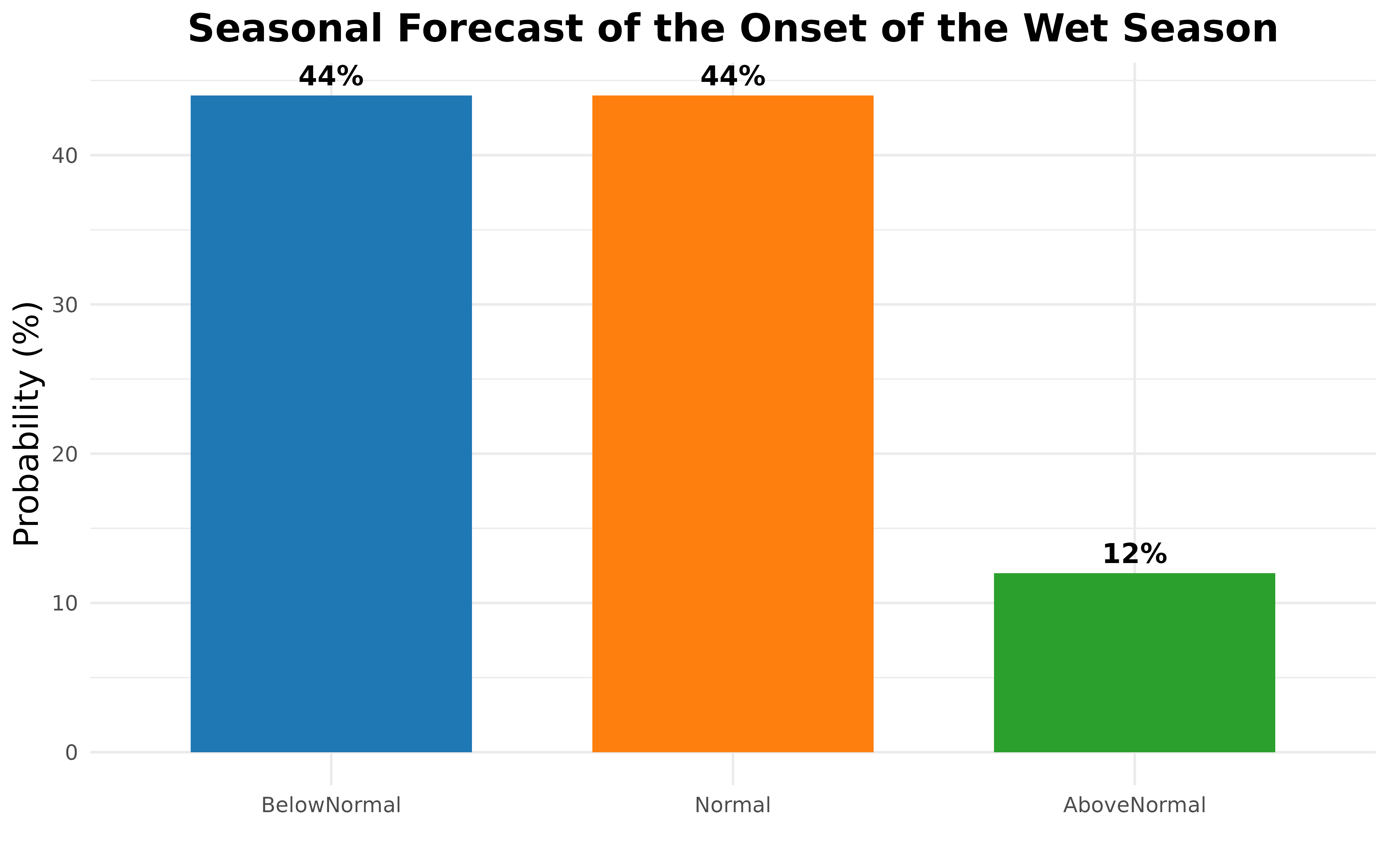
The seasonal forecast of the wet season calendar (WSC) variables i.e Onset and Cessation is produced by using tercile seasonal rainfall probabilities as input using using Quantile Bin Resampling (QBR) method. QBR is like the concept of analogue forecasting. With this resampling, historical WSC simulations are categorized by quantiles of seasonal rainfall totals associated with that season (e.g., upper, middle or lower tercile). Historical WSC outcomes can then be grouped according to these categories. This can transform probabilistic forecasts of rainfall quantiles into WSC forecast ensemble of any size. At last, the ensemble members are converted to WSC tercile probability.

Usage:

seasFcstQBR(hisYearStart, hisYearEnd, rainTerc, seasRain, hisWSCvar, fcstVarName, tercileMethod)

Example:

## Load example data:
data(AgroClimateData)

## Estimate daily PET:
PET <- calcEto(AgroClimateData, method = "PM", Zh = 10)

## Add the estimated PET 'ET.Daily' to a new column in AgroClimateData:
AgroClimateData$Eto <- PET$ET.Daily

## Estimate daily water balance for the soil having 100mm of WHC:
watBal.list <- calcWatBal(data = AgroClimateData, soilWHC = 100)
watBal <- watBal.list$data

## seasonal calendar is estimated for the onset window ranges from
## 01 September to 31 January having a soil with 100mm of WHC:

soilWHC <- 100
onsetWind.start <- "09-01"
onsetWind.end <- "01-31"
cessaWind.end <- "06-30"

seasCal.dF <- calcSeasCal(
  data = watBal, onsetWind.start, onsetWind.end,
  cessaWind.end, soilWHC
)

## Tercile Rainfall Probabilities of seasonal Forecast for OND, 2023:
rainTerc <- data.frame(T1 = 0.15, T2 = 0.10, T3 = 0.75)

## Summarize rainfall data for October to December:
seasRain <- AgroClimateData %>%
  filter(Month %in% c(10, 11, 12)) %>%
  group_by(Year) %>%
  summarize(sRain = sum(Rain))

## Start of the historical resampling year
hisYearStart <- 1991

## End of the historical resampling year
hisYearEnd <- 2022

## Historical WSC Simulations:
hisWSCvar <- seasCal.dF

## WSC variable to forecast:
fcstVarName <- "Onset"
tercileMethod <- "quantiles"

SeasFcst.dF <- seasFcstQBR(
  hisYearStart, hisYearEnd, rainTerc,
  seasRain, hisWSCvar, fcstVarName,
  tercileMethod
)


## Resafel the dataframe for ggplot:
SeasFcst.dFgg <- data.frame(
  Category = factor(
    c(
      "BelowNormal", "Normal",
      "AboveNormal"
    ),
    levels = c(
      "BelowNormal",
      "Normal",
      "AboveNormal"
    )
  ),
  Probability = c(
    (SeasFcst.dF$BelowNormal * 100),
    (SeasFcst.dF$Normal * 100),
    (SeasFcst.dF$AboveNormal * 100)
  )
)

## Create the bar plot:
ggplot(SeasFcst.dFgg, aes(x = Category, y = Probability, fill = Category)) +
  geom_bar(stat = "identity", width = 0.7) +
  scale_fill_manual(values = c(
    "BelowNormal" = "#1f77b4",
    "Normal" = "#ff7f0e",
    "AboveNormal" = "#2ca02c"
  )) +
  geom_text(aes(label = paste0(Probability, "%")),
    vjust = -0.5,
    size = 4, fontface = "bold"
  ) +
  labs(
    title = "Seasonal Forecast of the Onset of the Wet Season",
    x = " ",
    y = "Probability (%)"
  ) +
  theme_minimal() +
  theme(
    plot.title = element_text(hjust = 0.5, size = 16, face = "bold"),
    axis.title.x = element_text(size = 14),
    axis.title.y = element_text(size = 14),
    legend.position = "none"
  )

8. References

Allen, R.G.; Pereira, L.S.; Raes, D.; Smith, M. Crop Evapotranspiration: Guidelines for Computing Crop Water Requirements; FAO Irrigation and Drainage Paper no. 56; FAO: Rome, Italy, 1998; ISBN 92-5-104219-5.

Doorenbos, J. and Pruitt, W.O. 1975. Guidelines for predicting crop water requirements, Irrigation and Drainage Paper 24, Food and Agriculture Organization of the United Nations, Rome, 179 p.

FAO, 1977. Crop water requirements. FAO Irrigation and Drainage Paper No. 24, by Doorenbos J. and W.O. Pruitt. FAO, Rome, Italy.

FAO, 1986. Early Agrometeorological Crop Yield Forecasting. FAO Plant Production and Protection Paper No. 73, by M. Frère and G.F. Popov. FAO, Rome.

Hargreaves, G.H. and Samani, Z.A. (1985) Reference Crop Evapotranspiration from Temperature. Applied Engineering in Agriculture, 1, 96-99.

MacLeod D, Quichimbo EA, Michaelides K, Asfaw DT, Rosolem R, Cuthbert MO, et al. (2023) Translating seasonal climate forecasts into water balance forecasts for decision making. PLOS Clim 2(3): e0000138. https://doi.org/10.1371/journal.pclm.0000138

Priestley, C., & Taylor, R. (1972). On the assessment of surface heat flux and evaporation using large-scale parameters. Monthly Weather Review, 100(2), 81-92.

van den Dool HM. A New Look at Weather Forecasting through Analogues. Monthly Weather Review. 1989; 117(10):2230–2247. https://doi.org/10.1175/1520-0493(1989)117%3C2230:ANLAWF%3E2.0.CO;2

The Genetics Group at the Institute of Plant Sciences is a geographically and culturally diverse research team working on data-driven agricultural innovation combining crop genetics, climate, and participatory approaches. We are based at Scuola Superiore Sant’Anna, Pisa, Italy.

You can contact us sending an email to Matteo Dell’Acqua (mailto:m.dellacqua@santannapisa.it) or Mario Enrico Pè (mailto:m.pe@santannapisa.it). You can find out more about us visiting the group web page (http://www.capitalisegenetics.santannapisa.it/)

Robel Takele and Matteo Dell’Acqua

2024-09-26

1. Introduction

2. Installation and Loading

3. Required Climate Data

4. Potential Evapotranspiration

Usage:

Example:

5. Soil Water Balance

Usage:

Example:

6. Rainy Season Calendar

Usage:

Example:

7. Seasonal Forecast of WSC

Usage:

Example:

8. References